Blog
A recipe to solve (some) Stochastic Differential Equations analytically
I recently delved into the fascinating world of stochastic differential equations (in short SDEs) through an open MIT course. Amidst the richness of intriguing concepts, one particular point caught my attention and left me pondering. I felt like sharing this point with you.
The lecturer presented a recipe for solving SDEs analytically. They however said that this recipe would only work for a few SDEs, that in other cases it would fail and that instead you may have to feel the solution and verify it by plugging it into the SDE. They then went on saying that anyways, nowadays people would use computers to solve these equations.
If you share my enthusiasm for analytic solutions and have a desire to solve SDEs - even in a scenario where you might choose to reside in a secluded forest cabin devoid of electricity - then relying on a computer feels unsatisfactory.
While I am an admirer of verifying magically guessed solutions, I tend to forget relevant details of these it-makes-you-look-like-a-genius approaches.
So, I was thinking, can we extend the recipe so that it is useful for more SDEs, and in a way that is easy to memorize? If you wish to learn what I came up with, download the pdf version of this article with a click.
SST Standard Model Reinsurance - Computing the Insurance Risk with R
If you are an actuary and work for a reinsurance company licensed in Switzerland, you might have to calculate the Swiss Solvency Test (SST) Standard Model for reinsurers (StandRe). At the time of writing, the Swiss regulator FINMA provides two Excel templates that must be filed, one for computing the insurance risk (StandRe template) and one for aggregating insurance risk with financial risks (SST template).
The StandRe template splits the insurance risk into attritional events premium risk (AEP), attritional events reserve risk (AER), individual events related to pricing risk (IE1), individual events related to reserving risk (IE2) and natural catastrophe events (NE).
FINMA prescribes lognormal distributions for AEP and AER and compound Poisson - generalized Pareto distributions for IE1 and IE2. The main purpose of the StandRe template is to calibrate these distributions. With regards to defining a meaningful distribution for NE, FINMA currently leaves this task to the reinsurers.
The final step in completing the StandRe template is to compute and aggregate these distributions considering a t-copula dependency between AEP and AER ("the outputs of the components AE = AEP + AER, IE1, IE2 and NE are assumed to be independent prior to potential application of outward retrocession [..]" - FINMA 31 Jan 2021). We show how this final step can be done in R.
There are two R packages that seem to come in handy, actuar and copula. actuar provides functions to simulate compound frequency-severity distributions and copula gives us the t-copula.
There are several Pareto distributions available in actuar and we have to find which one corresponds to generalized Pareto distribution in the FINMA StandRe documentation.
According to the Technical description of StandRe, the CDF of the prescribed generalized Pareto is given by
\[ F(x) = 1 - \left(1 + \frac{\alpha_i}{\alpha_t}\left(\frac{x}{x_0}-1\right)\right)^{-\alpha_t} \] Substituting \(\theta = \alpha_tx_0/\alpha_i\) and \(\mu = x_0\), this expression becomes \[ \begin{eqnarray} F(x) &=& 1 - \left(\frac{\theta + x - \mu}{\theta}\right)^{-\alpha_t} \\ &=& 1 - \left(1 + (x - \mu)/\theta \right)^{-\alpha_t} \end{eqnarray} \] which corresponds to the Pareto II formulation in the R package actuar.
We are now ready to compute the insurance risk with R.
A Recipe in R
0) Model assumptions
In order to keep our example simple, we make the following assumptions.
- There is no natural catastrophe events risk NE (this can be easily added by means of an additional distribution to consider in the below lines of codes)
- There are only single model segments (modelling retrocession might require multiple model segments, but this is not the focus of this article)
- We ignore discounting (meaning we assume forward values = present values)
- The FINMA StandRe documentation as at Jan 2021 is still applicable
- The parameters of the distributions (AER, AEP, IE1 and IE2) have been estimated (which is the main purpose of the FINMA StandRe template)
1) Import parameters
We first import the values needed to simulate the non-life risk, define the parameters of the t-copula as prescribed by FINMA and set the number of simulations as well as a seed for reproducibility.
# IF ON A MOBILE, TURN THE SCREEN TO LANDSCAPE FOR READABILITY
# Import and define parameters
df_parameters           <- read.table(
                           file   = "standre.txt",
                           sep    = "\t",
                           header = TRUE)
rownames(df_parameters) <- df_parameters[,1]
t_rho                   <- 0.23
t_degreefreedom         <- 4.00
N                       <- as.integer(2.0e6)
set.seed(100)
The following table shows our invented parameters of the distributions which we are going to simulate.
| Parameter | AER | AEP | IE1 | IE2 |
|---|---|---|---|---|
| mu | 19.50 | 17.0 | - | - |
| sigma | 0.05 | 0.1 | - | - |
| freq | - | - | 2.2 | 0.5 |
| threshold | - | - | 1e6 | 1e6 |
| pareto_initial | - | - | 2.5 | 1.8 |
| pareto_tail | - | - | 5.0 | 3.0 |
2) Simulate IE1 and IE2
Second, we simulate the compound Poisson-Pareto distributions.
# Simulate IE1 and IE2
draw_ie <- data.frame(matrix(nrow = N, ncol = 2))
for(i in 1:2){
 model       <- paste0("IE", toString(i))
 theta       <- (df_parameters["pareto_tail", model]
                        * df_parameters["threshold", model]
                        / df_parameters["pareto_initial", model])
 draw_ie[,i] <- actuar::rcompound(N,
                 model.freq = stats::rpois(df_parameters["freq",model]),
                 model.sev  = actuar::rpareto2(
                      min   = df_parameters["threshold",model],
                      scale = theta,
                      shape = df_parameters["pareto_tail",model])
                 )
}
3) Simulate AER and AEP
Third, we draw from a 2-dimensional t-copula on which we apply the inverse lognormal CDFs to obtain draws for AER and AEP.
# Simulate AER and AEP
draw_ae           <- data.frame(matrix(nrow = N, ncol = 2))
colnames(draw_ae) <- c("R", "P")
draw_copula       <- copula::rCopula(
                      N,
                      copula::tCopula(
                      param   = t_rho,
                      dim     = 2,
                      df      = t_degreefreedom))
draw_ae[,"R"]     <- stats::qlnorm(
                      draw_copula[,1],
                      meanlog = df_parameters["mu", "AER"],
                      sdlog   = df_parameters["sigma", "AER"]
                      )
draw_ae[,"P"]     <- stats::qlnorm(draw_copula[,2],
                      meanlog = df_parameters["mu", "AEP"],
                      sdlog   = df_parameters["sigma", "AEP"]
                      )
In order to get an idea of the imposed dependency between AER and AEP, let's plot 2000 draws from the t-copula,

4) Aggregate the components and calculate key statistics
The 4th and final step is to aggregate the different distributions and calculate key statistics for the FINMA StandRe template (mean, standard devation, value at risk VaR(99%), expected shortfall ES(99%)). We also show the demeaned expected shortfall (we call it d-ES) as this corresponds to the definition of risk capital according to FINMA.
# Function to compute the results
compute_results <- function(draw_vector) {
    result_EL          <- mean(draw_vector)
    result_SD          <- sd(draw_vector)
    draw_sort          <- sort(draw_vector, decreasing = TRUE)[1:
                            as.integer(0.01 * length(draw_vector))]
    result_VaR         <- draw_sort[length(draw_sort)]
    result_ES          <- mean(draw_sort)
    result_d_ES        <- result_ES - result_EL
    return(c(result_EL, result_SD, result_VaR, result_ES, result_d_ES))
}
# Set up output data.frame
df_results <- data.frame(matrix(nrow = 5, ncol = 7))
colnames(df_results)   <- c("Total","AEP_IE1","AER_IE2","AEP","AER","IE1","IE2")
rownames(df_results)   <- c("MEAN","SD","VaR","ES","d-ES")
# Aggregate
aep_ie1                <- draw_ae[,"P"] + draw_ie[,1]
aer_ie2                <- draw_ae[,"R"] + draw_ie[,2]
total                  <- aep_ie1 + aer_ie2
# Compute results
df_results[,"IE1"]     <- compute_results(draw_ie[,1])
df_results[,"IE2"]     <- compute_results(draw_ie[,2])
df_results[,"AEP"]     <- compute_results(draw_ae[,"P"])
df_results[,"AER"]     <- compute_results(draw_ae[,"R"])
df_results[,"AER_IE2"] <- compute_results(aer_ie2)
df_results[,"AEP_IE1"] <- compute_results(aep_ie1)
df_results[,"Total"]   <- compute_results(total)
5) Dispay the results and conclude
We conclude by presenting a table with the aggregations 'Total' (= AEP + AER + IE1 + IE2), AEP + IE1 and AER + IE2. If we were to compute the entire SST, the next step would be to transfer the aggregated distribution 'Total' into the FINMA SST template, but this is out of scope of this article. Finally, we recommend to test the sufficiency of the number of simulations; for our example we used 2 million simulations and running it for the seeds 1, 100 and 200 resulted in variations in d-ES of the 'Total' distribution of less than 0.5%.
| Total | AEP + IE1 | AER + IE2 | |
|---|---|---|---|
| MEAN | 323.13 | 27.58 | 295.56 |
| SD | 15.75 | 3.44 | 14.83 |
| VaR | 361.94 | 36.70 | 331.74 |
| ES | 368.53 | 38.49 | 337.59 |
| d-ES | 45.40 | 10.91 | 42.04 |
Actuarial vs Financial Pricing - considering tradable insurance risks
Trading insurance risks has been made possible by innovations in the capital markets. It began in the 1990s when Catastrophe futures started trading on the Chicago Board of Trading (CBOT). And might be lifted to a whole new level by FinTech companies leveraging blockchains.
1) Traditional actuarial pricing
"There is no right price of insurance; there is simply the transacted market price which is high enough to bring forth sellers, and low enough to induce buyers".At university, I learned that tradable risks and non-tradable risks are priced differently. Traditional insurance risks have been considered as non-tradable, and financial instruments generally as tradable. In this view, the two text-book approaches areFinn and Lane (1997)
- No arbitrage
- Find a new probability measure Q by changing the real world probabilities in order to give more weight to unfavourable events
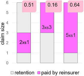
The actuarial price of two equal cash-flows, however, is not necessarily the same. As an example, consider two reinsurance alternatives for the same risk. Alternative 1, consisting of two XL treaties, 2xs1 and 3xs3. And an alternative 2, consisting of only one 5xs1 treaty. Obviously, these two alternatives produce the same cash-flows (assuming large enough annual aggregate limits). Nonetheless, the actuarial approach may result in two different prices for these alternatives. In our example below, alternative 1 costs 0.51 + 0.16 = 0.67 which is more than the cost of alternative 2, 0.64. Unthinkable for tradable risks.
2) Emergence of alternative risk transfer
In the 1990s, insurance-linked securities (ILS) emerged as a response to the reinsurance capital crunch following the 1992 Hurricane Andrew and 1994 Northridge Earthquake.ILS are only one component of the "alternative risk transfer" market. It is however out of the scope of this post to describe alternative risk transfer in more detail. The take-away of this section is that the market for alternative risk transfer is growing, weakening the non-tradability assumption for insurance risks.
3) Conclusion
For tradable insurance risks, a myopic traditional actuarial pricing is dangerous. It bears the risk of being arbitraged out of the market. There is ample literature on the financial approach to pricing insurance risks. See, for example, the papers of Delbaen and Haezendonck (1989), Sondermann (1991) and Embrechts (1996).
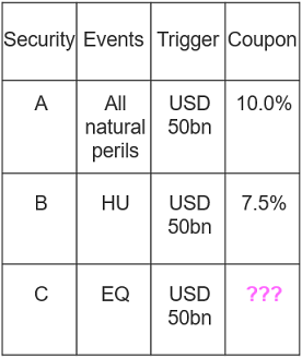
To conclude, let's do a pricing. Consider three (fictitious) securities with binary trigger based on industry loss, as depicted below. Security B, for example, pays the investor a coupon of 7.5% and suffers a complete loss if industry loss of a hurricane reaches USD 50bn. What coupon would you come up with for security C?
Can you guess the correlations?
Be it for portfolio analysis, an internal model or for pricing aggregate covers, modelling dependencies can be crucial. A popular concept is the one of correlations. However, correlations are indeed a very vague concept.
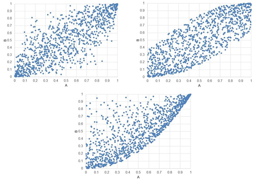
The following three graphs show simulated values of two random variables A and B. Instead of the values, their percentiles are plotted. The point (0.3, 0.5), for example, means the simulated values correspond to the 30th percentile for A and to the 50th percentile for B. For each graph, a correlation (Spearman's Rho) was used to produce the plots. Can you guess the values of these correlations?
The answer is...
The way to go is to use copulas instead of correlations. Contact us if you wish to know more about this subject.
Fun Articles about Mathematics
Getting my child to sleep. How do I do it optimally?
Let \(p(t)\) be the probability that the child wakes up when I try to leave after an amount \(t\) of time.
Let \(M\) be the value of one time unit of adult time. So leaving after \(t\) means a cost of \(M t\) (imagine, for example, having missed \(t\)-time of a movie, or of whatever adult activity you find pleasure in). Geekier parents may replace this linear function with a more general function \(M(t)\) but this won't really give us more insight as we will see.
Let \(E\) be an energy cost incurred from guilt feelings when your child wakes up (if you don't have these, imagine a small energy cost of having to return to your child).
The following assumptions describe my situation pretty well.
- ASSUMPTION 1. If I leave right away, my child wakes up for sure, so \(p(0)=1.\)
- ASSUMPTION 2. The longer I stay, the smaller this probability gets, which means, assuming differentiability, that the derivative of this function is negative, \(p'(t) \lt 0.\) To avoid nonsensical negative probabilities, \(p'(t)\) has to converge to zero with increasing \(t.\)
- ASSUMPTION 3. When my child wakes up upon a failed leave attempt, I have to start all over again, which is simplistically modelled as resetting the time \(t\) to zero. A cost of \(M t + E \) is incurred just before the reset.
The left-hand side is the price of waiting one more second versus leaving. Waiting a second longer means missing out one more time unit of adult time valued at \(M\), adult time which we could have enjoyed after a successful get away for which the probabilty is \(1-p(t)\). We observe that at \(t=0\) the price of waiting is zero because \(p(0)=1\) (by Assumption 1). It will increase with \(t\) (which is a consequence of Assumption 2).
The right-hand side is the value of waiting one more second versus leaving. Waiting a second longer decreases the probabilty of an unsuccessful escape by \(p'(t).\) In the event of an unsuccessful escape, \(E\) would incur and we would have to start all over again meaning losing an additional amount \(t\) of adult time valued at \(M t\) (in addition to the adult time we have already lost). We see that at \(t=0\) the value of waiting is positive because \(p'(0) \lt 0\) (by Assumption 2). Since \(p'(t)\) approaches zero with increasing \(t\), the value of waiting will eventually drop to zero.
To conclude, it's optimal to leave only if price and value of waiting are equal. Of course, every parent knows exactly when this is the case. This conclusion remains valid for more general \(M(t)\) but would have complicated things with a derivative of \(M(t)\) popping up along the way.
A quick test if a number is divisible by eleven
Separate the number at the decade position into two numbers as in the following three examples.
1) 1'199 becomes 11 and 99
2) 917'037 becomes 9'170 and 37
3) 264 becomes 2 and 64
If the sum of these two numbers is divisible by 11 then the original number can also be divided by 11.
It turns out that all of our examples are divisible by 11:
1) 11+99 = 110 is divisible by 11 and so is 1'199.
2) 9'170+37 = 9'207 is divisible by 11 because 92+07 = 99 is and therefore also 917'037 is divisible by 11.
3) 2+64 = 66 is divisible by 11 and so is 264.
A brief philosophy about transcendental numbers
We remember that the real numbers consist of rational (can be expressed as a fraction of two integers) and irrational (cannot be expressed as a fraction of two integers) numbers. An example of an irrational number is the square root of 2. Observe that squaring the square root of 2 gives us 2 which is rational. Not every irrational number yields a rational number when squared.
A transcendental number is an irrational number for which we cannot find a non-negative integer such that its power to that integer is rational. More exactly, a transcendental number is not a root of a finite, non-zero polynomial with rational coefficients. Pi is transcendental (the proof is not trivial, see Wikipedia) meaning that the square of Pi or Pi3 or Pi5 + 0.3*Pi2 etc. are all irrational. A number which is not transcendental is called algebraic. 0.25 is algebraic. The square root of 2 is also algebraic.
Pi being transcendental is the reason why squaring the circle is impossible, a problem which kept ancient geometers busy. Indeed, if it were possible to square a circle meaning that we could construct a square with the same area as a circle using only a finite number of steps with a circle and a straightedge then this would imply the existence of a polynomial for which Pi is a root which is a contradiction (intersecting lines and circles boils down to equating polynomials).
Where can we find transcendental numbers? Well, take any two different numbers and there is an infinity of transcendental numbers between them. Proof: Pi is transcendental and so is q*Pi for any rational q not equal to zero (because if q*Pi were not transcendental then it would be the root of a polynomial with rational coefficients which would automatically make Pi algebraic too which is a contradiction) and there is an infinity of q so that q*Pi lies between our two numbers.